Matplotlib 学习笔记

安装

随便找了一个教程，这部分很简单，没有大问题

基本用法

import matplotlib.pyplot as plt
import numpy as np
x=np.linspace(-1,1,50)
y1=x**2
plt.plot(x,y)
plt.show()

figure 图像

• plt.figure(num=3,figsize=(8,5)) num表示序号，是第几个图，figsize表示大小，长和宽
• plt.plot(x,y1,color='red',linewidth=5.0,linestyle='--') color表示线的颜色，linewidth表示线的宽度，linestyle表示类型，虚线用--表示

设置坐标轴

• plt.xlim((-1,2)) plt.ylim((-1,3)) 设置x或y轴的取值范围
• plt.xlabel('x') plt.ylabel('y') 设置坐标轴表示
• new_ticks=np.linspace(-1,2,5)
• plt.xticks(new_ticks) 设置坐标轴的值
• plt.yticks([-2,-1.8,-0.5,1,2],[r'$a\ \alpha c$',r'$b$',r'$c$',r'$d$',r'$e$'])设置坐标轴的值和标识
• ax = plt.gca() 图像的边框

legend 图例

l1, = plt.plot(x,y2,label='up')
l2, = plt.plot(x,y1,color='red',linewidth=1.0,linestyle='--',label='down')
plt.legend(handles=[l1,l2],labels=['aaa'],loc='best')

handles表示需要legend的线条，labels表示legend中线条的名称，loc表示位置，best可以自动选区最好的位置。

annotat 注解

import numpy as np
import matplotlib.pyplot as plt
x= np.linspace(-3,3,50)
y=2*x+1
plt.figure(num=1,figsize=(8,5))
plt.plot(x,y)

ax=plt.gca()
ax.spines['right'].set_color('none')
ax.spines['top'].set_color('none')
ax.spines['top'].set_color('none')
ax.xaxis.set_ticks_position('bottom')
ax.spines['bottom'].set_position(('data',0))
ax.yaxis.set_ticks_position('left')
ax.spines['left'].set_position(('data',0))

x0=1
y0=2*x0+1
plt.scatter(x0,y0,s=50,color='r')
plt.plot([x0,x0],[y0,0],'k--',lw=2.5,color='b')

#method 1
plt.annotate(r'$2x+1=%s$' % y0, xy=(x0,y0),xycoords='data',xytext=(+30, -30), textcoords='offset points',fontsize=16,arrowprops=dict(arrowstyle='-',connectionstyle='arc3,rad=0.2'))

# method 2
plt.text(-3.7,3,r'$This\ is\ the\ some\ text. \mu\ \sigma_i\ \alpha_t$',
         fontdict={'size': 16, 'color': 'b'})
plt.show()

tick 能见度

for label in ax.get_xticklabels() + ax.get_yticklabels():
    label.set_fontsize(12)
    # set zorder for ordering the plot in plt 2.0.2 or higher
    label.set_bbox(dict(facecolor='white', edgecolor='none', alpha=0.8, zorder=2))

注意dict中的参数zorder表示是哪一个图层

scatter 散点图

import matplotlib.pyplot as plt
import numpy as np

n = 1024    # data size
X = np.random.normal(0, 1, n)
Y = np.random.normal(0, 1, n)
T = np.arctan2(Y, X)    # for color later on
plt.scatter(np.arange(5),np.arange(5))

# plt.scatter(X, Y, s=75, c=T, alpha=.5)
# plt.xlim(-1.5, 1.5)
plt.xticks(())  # ignore xticks
# plt.ylim(-1.5, 1.5)
plt.yticks(())  # ignore yticks

plt.show()

X,Y是由numpy产生的随机数组，c为颜色模式，alpha为能见度

Bar 柱状图

import matplotlib.pyplot as plt
import numpy as np
n=12
X=np.arange(n)
Y1=(1-X/float(n))*np.random.uniform(0.5,1.0,n)
Y2=(1-X/float(n))*np.random.uniform(0.5,1.0,n)

plt.bar(X,+Y1,facecolor='r',edgecolor='white')#打印柱状图，正负表示方向
plt.bar(X,-Y2,facecolor='b',edgecolor='yellow')

for x,y in zip(X,Y1):
    plt.text(x,y,'%.2f' % y,ha='center',va='bottom')#注释值
for x, y in zip(X, Y2):
    plt.text(x , -y , '%.2f' % y, ha='center', va='top')
plt.show()

Contours 等高线图

import matplotlib.pyplot as plt
import numpy as np
def f(x,y):
    return (1-x/2+x**5+y**3)*np.exp(-x**2-y**2)
n=256
x=np.linspace(-3,3,n)
y=np.linspace(-3,3,n)
X,Y = np.meshgrid(x,y)

# 画图
plt.contourf(X,Y,f(X,Y),8,alpha=0.75,cmap=plt.cm.hot)

# 线条
C=plt.contour(X,Y,f(X,Y),8,colors='black',linewidth=.5,alpha=0.5)

# 线条数值
plt.clabel(C,inline=True,fontsize=10)

plt.xticks(())
plt.yticks(())
plt.show()

image图片

import matplotlib.pyplot as plt
import numpy as np

# image data
a = np.array([0.313660827978, 0.365348418405, 0.423733120134,
              0.365348418405, 0.439599930621, 0.525083754405,
              0.423733120134, 0.525083754405, 0.651536351379]).reshape(3,3)

"""
interpolation的官方参数网站，表示图像的类型样式
for the value of "interpolation", check this:
http://matplotlib.org/examples/images_contours_and_fields/interpolation_methods.html
for the value of "origin"= ['upper', 'lower'], check this:
http://matplotlib.org/examples/pylab_examples/image_origin.html
"""

plt.imshow(a, interpolation='nearest', cmap='hot', origin='upper')
plt.colorbar(shrink=1)

plt.xticks(())
plt.yticks(())
plt.show()

3D plot

import numpy as np
import matplotlib.pyplot as plt
from mpl_toolkits.mplot3d import Axes3D
fig = plt.figure()
ax = Axes3D(fig)
X=np.arange(-4,4,0.25)
Y=np.arange(-4,4,0.25)
X,Y=np.meshgrid(X,Y)
R = np.sqrt(X**2+Y**2)
Z=np.sin(R)
# 行跨，列跨
ax.plot_surface(X,Y,Z,rstride=1,cstride=1,cmap=plt.get_cmap('rainbow'),edgecolor='black')
# rstride表示跨行长度,cstride表示列跨长度,cmap表示颜色样式,edgecolor行跨列跨的线条

# 投影图，zdir表示投影到的坐标平面，offset表示所在平面的位置，cmap表示颜色样式
ax.contourf(X,Y,Z,zdir='y',offset=4,cmap='rainbow')
# Z平面的位置
ax.set_zlim(-2,2)

plt.show()

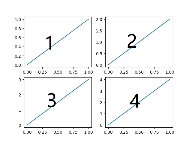
subplot多个显示

# plt.subplot(行，列，位置序号)
import matplotlib.pyplot as plt

plt.figure()

plt.subplot(2,2,1)
plt.plot([0,1],[0,1])

plt.subplot(2,2,2)
plt.plot([0,1],[0,2])

plt.subplot(2,2,3)
plt.plot([0,1],[0,3])

plt.subplot(2,2,4)
plt.plot([0,1],[0,4])

plt.show()

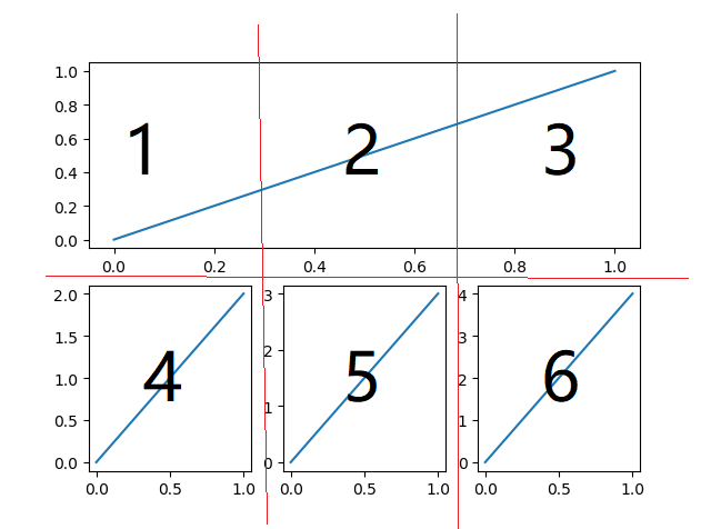
import matplotlib.pyplot as plt

plt.figure()

plt.subplot(2,1,1)
plt.plot([0,1],[0,1])

plt.subplot(2,3,4)
plt.plot([0,1],[0,2])

plt.subplot(2,3,5)
plt.plot([0,1],[0,3])

plt.subplot(2,3,6)
plt.plot([0,1],[0,4])

plt.show()

subplot 分格显示

method 1:subplot2grid

import matplotlib.pyplot as plt
plt.figure()
ax1=plt.subplot2grid((3,3),(0,0),colspan=3,rowspan=1)
ax1.plot([1,2],[1,2])
ax1.set_title("ax1")
ax2=plt.subplot2grid((3,3),(1,0),colspan=2)
ax2.plot([1,2],[1,2])
ax3=plt.subplot2grid((3,3),(2,0),colspan=1)
ax3.plot([1,2],[1,2])
ax4=plt.subplot2grid((3,3),(1,2),rowspan=2)
ax4.plot([1,2],[1,2])
ax5=plt.subplot2grid((3,3),(2,1))
ax5.plot([1,2],[1,2])

plt.subplot2grid((3,3)表示形状,(2,1)图像左上角的位置,colspan=3 所占列,rowspan=1所占行)

method 2:gridspec

import matplotlib.pyplot as plt
import matplotlib.gridspec as gridspec
plt.figure()
gs=gridspec.GridSpec(3,3)
ax1=plt.subplot(gs[0,:])#所占行索引，所占列位置索引
ax2=plt.subplot(gs[1,:2])
ax3=plt.subplot(gs[1:,2])
ax4=plt.subplot(gs[-1,0])
ax5=plt.subplot(gs[-1,-2])# 负数表示倒数第几个索引

method 3:easy to define structure

import matplotlib.pyplot as plt
f,((ax11,ax12),(ax21,ax22))=plt.subplots(2,2,sharex=True,sharey=True)
ax11.scatter([1,2],[1,2])

传出的f可以用来调整窗口的格式，share表示是否共享坐标轴，

图中图

import matplotlib.pyplot as plt

fig = plt.figure()
x=[1,2,3,4,5,6,7]
y=[1,3,4,2,5,8,6]

left,bottom,width,height=0.1,0.1,0.8,0.8
ax1=fig.add_axes([left,bottom,width,height])
ax1.plot(x,y,'r')
ax1.set_xlabel('x')
ax1.set_ylabel('y')
ax1.set_title('title')

left,bottom,width,height=0.2,0.6,0.25,0.25
ax2=fig.add_axes([left,bottom,width,height])
ax2.plot(y,x,'b')
ax2.set_xlabel('x')
ax2.set_ylabel('y')
ax2.set_title('title inside 1')

plt.axes([0.6,0.2,0.25,0.25])
plt.plot(y[::-1],x,'g')
plt.xlabel('x')
plt.ylabel('y')
plt.title('title inside 2')

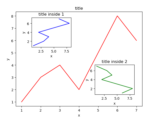
其实就是用行列位置+宽高尺寸所确定的绝对位置来布置图片，这里的尺寸是图片占窗口的百分比

次坐标轴

import matplotlib.pyplot as plt
import numpy as np
x = np.arange(0,10,0.1)
y1=0.05*x**2
y2=-1*y1

fig,ax1=plt.subplots()
ax2 = ax1.twinx()
ax1.plot(x,y1,'g-')
ax2.plot(x,y2,'b--')

ax1.set_xlabel('X data')
ax1.set_ylabel('Y1',color='g')
ax2.set_ylabel('Y2',color='b')

animation 动画

import numpy as np
from matplotlib import pyplot as plt
from matplotlib import animation

fig ,ax=plt.subplots()
x=np.arange(0,2*np.pi,0.01)
line,=ax.plot(x,np.sin(x))

def animate(i):#传进去的是frames
    line.set_ydata(np.sin(x+i/100))
    return line,
def init():
    line.set_ydata(np.sin(x))
    return line,
ani = animation.FuncAnimation(fig=fig,func=animate,frames=1000,init_func=init,interval=20,blit=True)
#  init表示初始状态,animate表示过程状态，方法传入值为frames，frames表示一共有多少帧，interval表示一帧停留多少（毫秒）
plt.show()

许多方法参数还需要在未来实践中慢慢摸索，matplotlib是真滴强大！！！Orz Orz Orz Orz Orz